Demystifying EEG Microstates

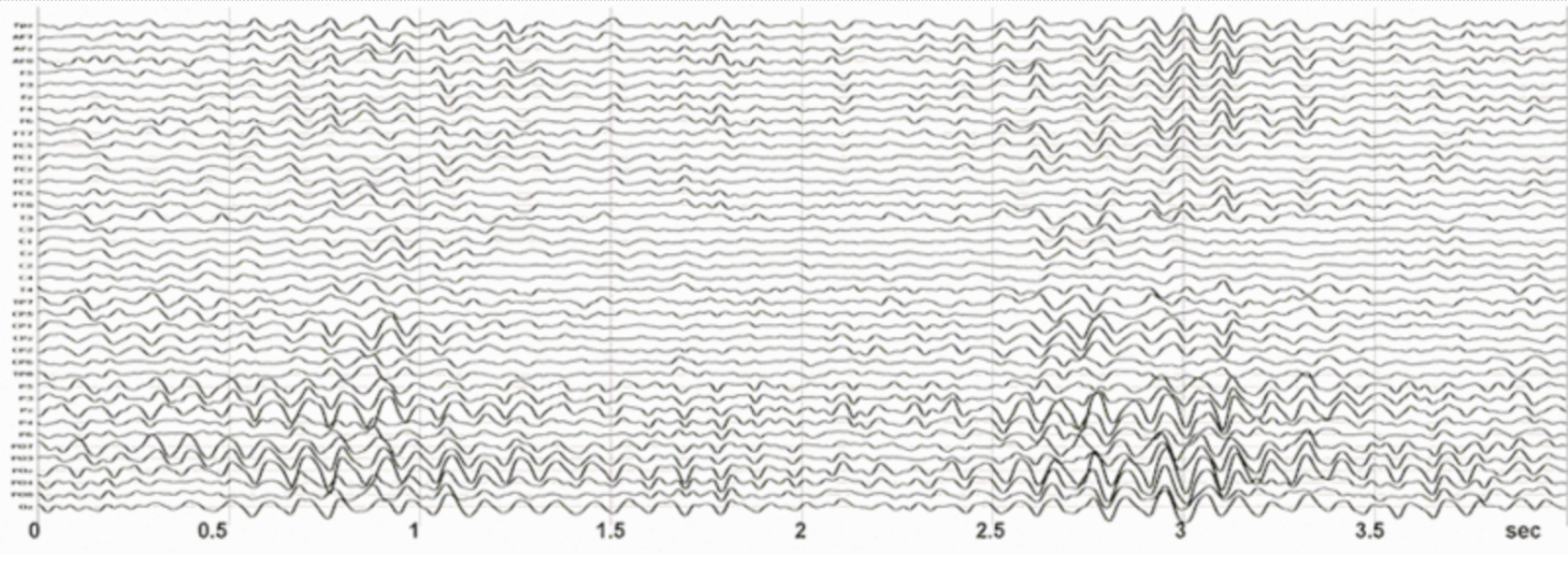
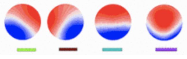
EEG Microstates allow for a sparse characterisation of spatial and temporal features of large scale brain network activity. EEG Microstates, also nicknamed as “the atoms of thought”, are transient, patterned and quasi stable states of EEG.

• Transient: They exist only for a short time duration (Durations of microstates during spontaneous task-free resting EEG on average are in the range of 70 to 125 milliseconds) - Patterned - Observable and noticeable
• Quasi Stable - Global topography is fixed, but strength might vary and polarity invert.

Pascual et al. Segmentation of brain electrical activity into microstates: model estimation and validation [LINK]

Microstate EEGlab toolbox: An introductory guide [Tutorial Implementation]
Credits: The code was published in the Tutorial by Poulsen et al.

Analysis Methodologies

* Consider this EEG time series with 32 electrodes sampled at every ‘x’ seconds. For this time series we have ‘x’ EEG states which are [32x1] vectors.

* We now have a topographical map corresponding the EEG states.

* We start with choosing n (here = 4) random template maps. Then we use the k-means clustering algorithm to cluster or classify the EEG state maps into one of the n microstates.

* After the EEG states have been assigned to a microstate, we see the EEG time series also classified to different (n) microstates. Here we see only one channel data as the above series only shows the GFP

Global Field Power

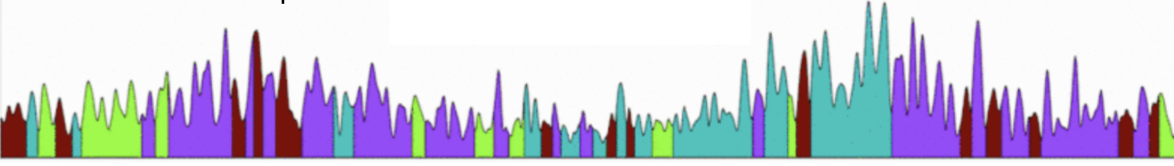
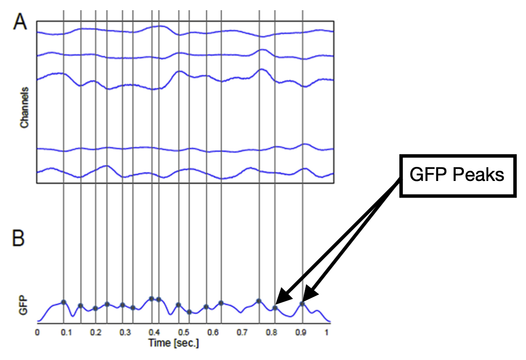
• GFP (Global Field Power) - quantifies the amount of activity at each time point in the field considering the data from all recording electrodes simultaneously.

* The measure of global field power (GFP) corresponds to the spatial standard deviation, and it quantifies the amount of activity at each time point in the field considering the data from all recording electrodes simultaneously resulting in a reference-independent descriptor of the potential field. We use L1 norm to calculate the GFP peaks.

Where,
~ K - number of channels
~ V(t) - EEG state represented by a (K x 1) vector

Analysis Algorithm

{In most scenarios, number of EEG recording channels (Ns) >> number of microstates (Nµ) as with EEG microstates we are trying to represent an EEG time-series with the least possible number of states.}

• Let us consider a model with just 2 EEG recording channels (Ns = 2). Thus we have a 2-D plane that represents all possible electric potential values, and a single point corresponds to an instantaneous measurement.

• For a classification model to be effective, it needs to have a minimum of 2 clusters, thus in this scenario we have 2 microstates. (Nµ = 2)

• Now, we initialize the two brain microstates as random vectors which are at unit distance from the origin. All points lying on the line going from the origin toward the microstate belong to the same microstate.

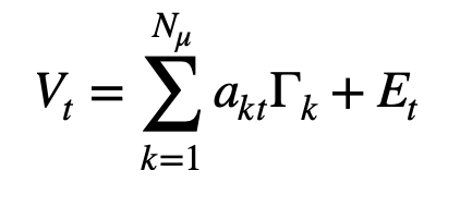
• In mathematical terms the final aim for microstate analysis is,

Where,
~ Vt = (Ns x 1) vector consisting of the scalp electric potential measurements
~ Γk = is the normalised Ns x 1 vector representing the kth microstate
~ akt = the kth microstate intensity at time instant t.

• Moreover, every EEG state can only be represented by just one microstate i.e. in order to allow for non-overlapping microstates at each time instant t, all akt must be zero except for one. Therefore, at each time instant, the summation reduces to a single nonzero term, corresponding to a single active microstate.

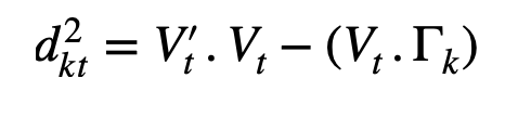
• Now, the above mentioned equation will not be able fit perfectly especially when (Ns >> Nµ) or when the EEG time series is long ie. we have many EEG states. Thus we add a term for error.

* The goal will be find microstates such that
1. Every EEG state will belong to only one microstate
2. The total error in the system will be minimum. The orthogonal squared distance between each measurement vector and microstate is computed. The higher the distance the higher the error.

* Let us assume we now have 32 electrodes and choose to classify them into 4 microstates.
1. We have a 32 dimension space, with every point a possible EEG state. Dimension of the EEG state here is 32x1.
2. We randomly construct random vectors in the above mentioned space of unit length. The dimension of the microstate is 32x1.
3. We now use k-means algorithm which gives the 4 most optimal microstates; and classifies all EEG states into one of those microstates with the orthogonal squared distance (error) less than the threshold error which was set by the user.

Directory Structure

• src folder contains the source code.

Running the code

Any changes which need to be made, must be made in the code block under the heading "Main" only

1. Run the code which launches the GUI based environnment.
2. Draw a rectagle around the region to be kept using right mouse button.
3. Next you can mark refinment storkes - Mark with these keys 0 (background) and 1 (foreground).